Tour of Temporal: Performance

In the last part of this series, we looked into the fundamentals of the Temporal workflow engine and how it compares to actor toolkits such as Akka. As I wrote in the previous part, my personal experience with workflows has led me to associate anything with the word “worfklow” in it to “a slow process” (taking minutes to complete). In order to clear that idea from my mind (and also because I like exploring performance characteristics of technologies) I wanted to have a closer look at the performance of Temporal workflows.

In this article we are going to look at various ways to execute the Payment Handling Worfklow example, measuring the latency of a workflow run at the call site. For all things throughput I invite you to have a look at Maru, a load testing tool for temporal workflows.

Experimental setup

The Temporal server uses a database to store its state, so for a latency test the only real bottleneck would be disk I/O (given a machine with enough CPU and memory). I therefore opted to run the benchmark on one of my machines which would allow me to eliminate the network as a source of latency / of inconsistencies between runs.

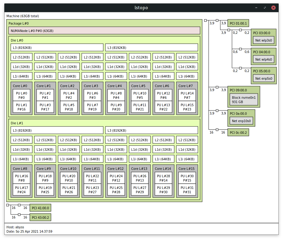
The machine in question has an AMD Ryzen Threadripper 1950X 16-Core processor, 64 GB of RAM and a Samsung SM961 NVMe SSD (sequential write of ~ 1800 MB/s), as shown below:

I used the docker-compose Temporal configuration with PostgreSQL as a database server.

The benchmark itself is carried out using JMH (the Java Microbenchmark Harness) with the following setup:

 1
 2
 3
 4
 5
 6
 7
 8
 9
10
11
12
13
14

public class PaymentHandlingWorkflowBenchmark {

    @Benchmark
    @BenchmarkMode({Mode.SampleTime})
    @OutputTimeUnit(TimeUnit.MILLISECONDS)
    @Warmup(iterations = 1)
    @Measurement(iterations = 10, time = 10)
    @Fork(value = 1, warmups = 0)
    public PaymentResult latencyBenchmark(WorkflowSetup setup) {
        PaymentHandlingWorkflow workflow = setup.client.newWorkflowStub(PaymentHandlingWorkflow.class, WorkflowOptions.newBuilder().setTaskQueue(Shared.COMMON_TASK_QUEUE).build());
        return workflow.handlePayment(new OrderId(UUID.randomUUID().toString()), setup.amountToSpend, setup.merchantId, setup.userId);
    }

}

Some notes on the JMH configuration:

• this setup will sample the latency of the workflow execution over 10 runs, giving 10 seconds to each run (for the baseline topology this means roughly ~2000 executions)
• setting up the workflow state (i.e. client connections, workers, etc.) is done once per benchmark run, we only benchmark a workflow execution
• given the resulting latencies there isn’t much sense to do much warmup (we’re in the hundreds of ms range). Warmups are used on the JVM since it requires - well - a bit of time to warm up.

Workflow and activities topologies

In order to get a good picture of the impact of different topologies, I ran the benchmark with the following setup:

• one worker node with main workflow and child workflow
• one worker node with main workflow an child workflow, using local activities
• one worker node using one (merged) workflow
• one worker node using one (merged) workflow and local activities
• two worker nodes with one (merged) workflow and local activities
• two worker nodes with one (merged) workflow and dedicated activity workers

For a latency benchmark, configuring more shards doesn’t make that much more sense, also thanks to a feature of Temporal that we’re going to discuss later.

Before going further, let’s examine a bit these topologies.

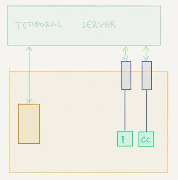
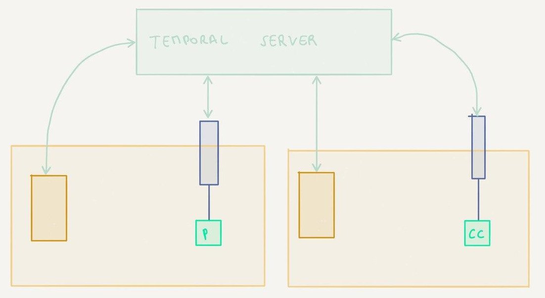
One worker node, parent and child workflows

This is the setup from the previous article. The main workflow executes the overall payment, the child workflow executes the part specific to each payment method (a credit card payment in this example).

I deliberately chose to use a child workflow in the example for two reasons:

• code organization: different payment handling methods get their own separate workflows and activities
• routing: for the payment processing example, the activities for one specific acquirer bank could be executed on a particular host, which is sometimes a requirement in real life (because only that host is allowed to communicate with the host of the bank)

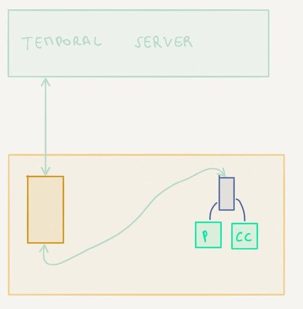
One worker node, parent and child workflows, local activities

This is essentially the same topology as previously with one important difference: both activities are configured as local activities.

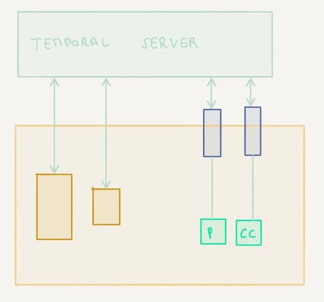
With normal activities, the workflow worker reports back to the Temporal server when it is time to execute activities. It is then the Temporal server that instructs an activities worker registered for this activities to carry them out. The result is persisted by the Temporal server before it hands the execution flow back to the workflow worker.

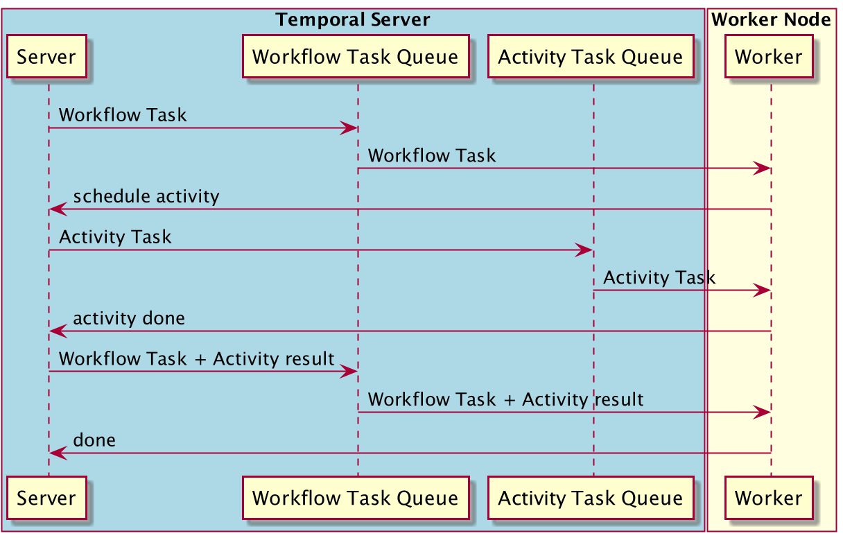
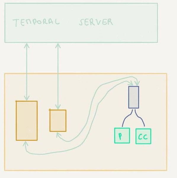
With local activities, the Temporal server instructs a workflow worker node to start a workflow execution, as it would do with normal activities. The difference lies in the execution of the activities: instead of passing back the control to the Temporal server, the worker node will directly run the activities using a local activity task queue. Once the entire workflow is executed, the results of the workflow and of each activity execution are reported back to the Temporal server.

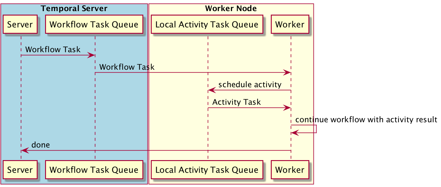
As you can imagine, the second scenario is going to lead to slower executions overall given the additional steps involved (network and persistence). Local activities are designed to be used for tasks that execute quickly and do not require advanced queuing or routing semantics.

One worker node, one workflow

In this setup, the two workflows are combined into one. Instead of calling a child workflow, we just call a method.

One worker node, local activities

Same as above but with local activities. This is the “smallest” topology there is.

Two worker nodes with one workflow

In this setup, there are now two worker nodes each capable of executing the workflow and the activities.

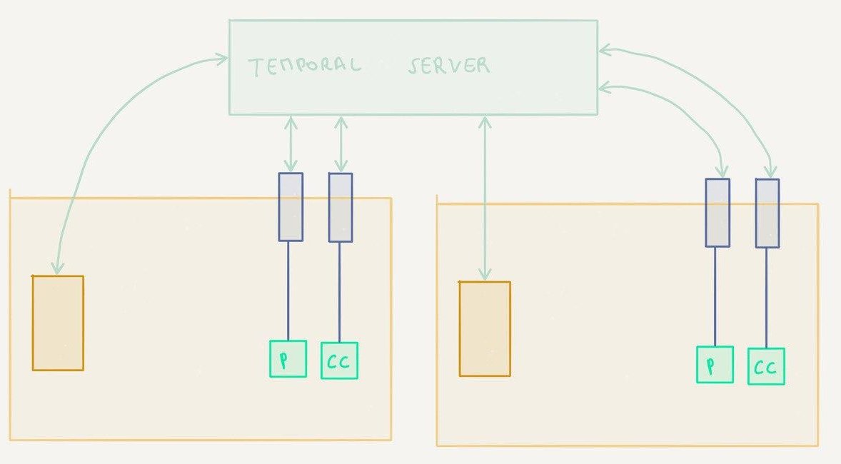
Two worker nodes with one workflow and dedicated activity workers

In this setup, the workers only register one of the two activities instead of both

Results

Without further ado, let’s have a look at the results:

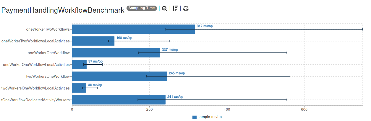
So what to make of this? There are several interesting observations here (click on the image to explore the results in detail):

• using child workflows definitely carries some overhead in comparison to using just one workflow (~90 ms with this setup). This is to be expected, since the execution is handed back to the Temporal server so there are more coordination efforts involved.
• the best result is achieved when using one workflow and local activities (as expected, I would say). Continuing the analogy with actors from the previous part, I’d say that this is what comes closest to the idea of an actor (the main difference still being that the supervision is left to the remote Temporal server)
• using dedicated workers per activity type doesn’t have any significant impact here — mainly, I should say, because the activities don’t really have any distinguishing characteristics. If they did carry out operations that could benefit from locality (i.e. having data around on the same worker machine) we could probably have observed better results with this type of routing.
• talking about locality, I think that it is important to mention at this point that Temporal uses an optimization for “sticky” workflow execution, i.e. workflow caching. When executing a workflow and resuming the workflow after running activities on another worker node, the server will hand back the execution to the workflow worker instance that initially started the workflow. This way, any previous results and state about that workflow can be re-used without the need for them to be passed on from the server to the worker node (which would happen in case of a crash of the workflow node, for example).

One more thing: looking at the results it may be tempting to think about using local activities as a way to make things faster. Unless you do have a use-case that does require lower latencies, I would recommend against it. In fact it is very likely that for a vast majority of workflows out there such low latencies aren’t required and being able to shard out activities execution (or individually throttle it) is more important than gaining a bit of time. I’ll discuss this topic at more length later in this series.

Conclusion

In this part of the series we compared the execution speed of several workflow deployment topologies and I think it is safe to say that modern workflow orchestration engines like Temporal can be quite snappy.

In the next series we will go back to exploring core concepts of Temporal such as event handling, queries and scheduling.